MV-2040: Load Estimation for a Fore Canard Actuator Mechanism Under Aero-dynamic
Loads
In this tutorial, you will learn how to represent pressure/distributed loads as Modal
Forces on a CMS flexible body and scale Modal Forces to real world loads in MotionView/MotionSolve.
Forces acting on a flexible body may be an aerodynamic load, liquid pressure, a
thermal load, an electromagnetic force or any force generating mechanism that is
spread out over the flexible body, such as non-uniform damping or visco-elasticity.
It may be even a contact force between two bodies. These distributed loads can be
conveniently transformed from Nodal to Modal domain and represent as Modal
Forces.
If we define as the mode shapes of the flexible body, and as the Nodal load acting on the flexible body, the
equivalent Modal load on the flexible body is defined as:
In this exercise, you will create a flexible body of a Fore Canard of an
aircraft with aerodynamic loads using OptiStruct.
Aero-dynamic loads for three operating positions of the fore canard, namely -10 deg,
0 deg, and 10deg, considering an air speed of 200m/sec at 1 atm pressure are
available from a CFD simulation using AcuSolve. A later
section of the exercise involves embedding this flexible body in the actuator
mechanism model in MotionSolve to estimate actuator
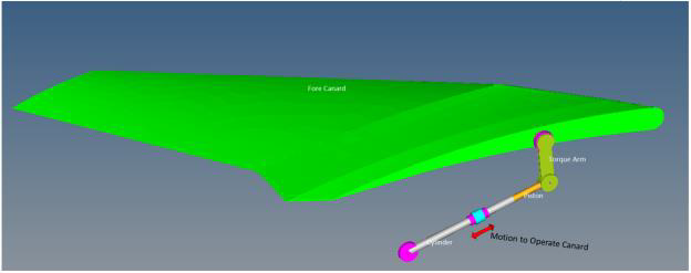
loads required for the operation of fore canard. Figure 1. Fore Canard of an Aircraft
Create a Fore Canard Flexible Body
In this step, you will create the Fore Canard flexible body.
Before you begin, copy all of the files located in the
mbd_modeling\flexbodies\modalforce folder to the
<working directory>.
Open ForeCanard.hm in HyperMesh with OptiStruct selected as the user
profile.
Review the model.
Figure 2.
The HM file contains a meshed model of Fore Canard with material
properties and control cards defined.
Figure 3. HyperMesh Model Browser
Note: Model units are Newton-Meter-KG-Sec, therefore all properties
defined are consistent with this unit system.
Create aerodynamic loads from CSV files.
Average pressure distribution over the surface of canard is exported as text
file from AcuFieldView. This file contains the
location and value of the pressure. The
AerodynamicLoad_0deg.csv,
AerodynamicLoad_Negative10deg.csv, and
AerodynamicLoad_Positive10deg.csv files contain the pressure
distribution information for 0deg, -10 deg, and 10 deg of canard orientation
respectively.
Add load collectors for three cases:
Left-click on the Load Collector icon from the toolbar.
In the panel, verify that the create radio
button is selected.
Specify the new load collector name as
AerodynamicLoad_0deg.
In the drop-down menu, select no card
image.
Click Create.
Figure 4.
Follow steps 3.a through 3.e to
create two more load collectors named
AerodynamicLoad_Negative10deg and
AerodynamicLoad_Positive10deg.
Click Return.
Browse to the Pressure load panel.
Click the Analysis radio button.
On the Analysis page, click on the Pressure
button.
Figure 5.
This will open the pressure panel.
Set the pressure load type to linear
interpolation.
Verify that the create radio button is
selected.
Figure 6.
Next to the faces button, click the drop-down
arrow. Change the surface selection type from faces to
elems.
Figure 7.
Figure 8.
In the magnitude drop-down menu, click linear
interpolation.
Figure 9.
Figure 10.
Now you can select elements on which pressure loads are applied and a
CSV file for pressure load info. Figure 11.
Create pressure loads on a canard surface.
Pressure loads for each position are created under their respective load
collectors so you can scale them in MotionSolve with
respect to the canard position.
Left-click on Set Current Load Collector.
Figure 12.
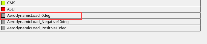
From the load collector list, choose
AerodynamicLoad0_deg.
Figure 13.
This will set AerodynamicLoad_0deg as the current load
collector.
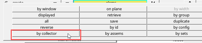
Click the elems button. Select by
collector from the list.
Figure 14.
Figure 15.
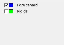
From the component collector list, click Fore
Canard. Click the select button
to return to the pressures panel.
Figure 16.
Click the ellipse button to browse for a
file.
.
Figure 17.
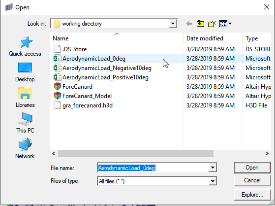
In the Open dialog, browse your
<working directory> and select
AerodynamicLoad_0deg.csv. Then click
Open.
Figure 18.
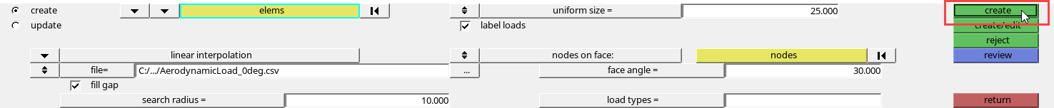
Click create to create pressure loads for the
0deg position.
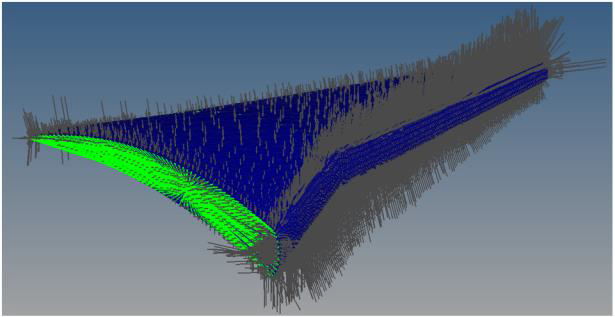
Figure 19.
Figure 20.
Note: The pressure load on each element is obtained by a linear
interpolation of pressure values with respect to its
location.
Follow step 6 again to create pressure loads for the
AerodynamicLoad_Negative10deg and AerodynamicLoad_Positive10deg load
collectors.
Specify load sets for CMS method.
Three load cases modeled in previous step represent nodal forces. These nodal
forces are transformed as modal forces using CMS method. In this step you modify
the existing CMSMETH card image to include three load sets.
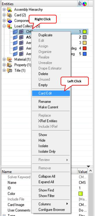
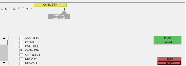
In the Entities browser, right-click on the CMS
load collector.
In the context menu, click Card
Edit.
Figure 21.
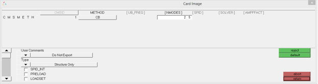
This will open the load collector card image. Figure 22.
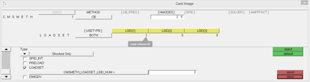
Specify load sets for CMSMETH.
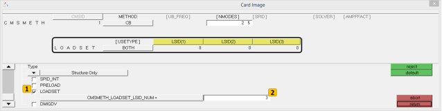
In the Card Image dialog, activate the
LOADSET checkbox.
Specify the CMS_LOADSET_LSID_NUM value as
3.
Figure 23.
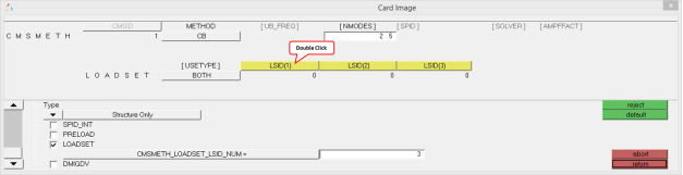
The card image shows an option to specify three load sets.
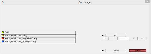
Double-click LSID(1).
Figure 24.
From the load collectors list, click
AerodynamicLoad_0deg. Click the
return button to go back to the CMS card
image.
Figure 25. Figure 26.
Use steps 8.c and 8.d to
specify AerodynamicLoad_Negative10deg for LSID(2)
and AerodynamicLoad_Positive10deg for
LSID(3).
Click Return.
Generate flexbody.
Your model is now ready for solving to generate a flexbody. The two control
cards required to solve for flexbody creation are already specified in the
model.
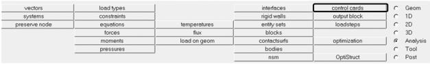
On the Analysis page, click on control cards
button.
Figure 27.
Click on the DTI_UNITS button from the first
page to review flexible body units. Then click
Return.
Figure 28.
In the next card, click on GLOBAL_CASE_CONTROL
to see the CMS load collector specified for CMSMETH solution. Click
return twice.
Figure 29.
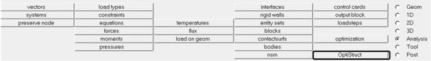
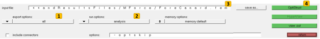
From the Analysis page, click on
Optistruct.
Figure 30.
In the panel, set the following options:
Set export options to all.
Set run options to analysis.
Browse to your <working directory> and
specify input file name as
flex_ForeCanard.fem.
Click on the Optistruct button.
Figure 31.
This will solve the model.
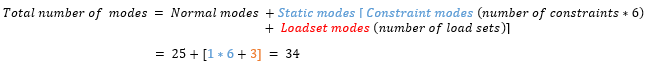
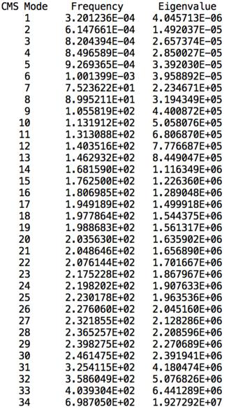
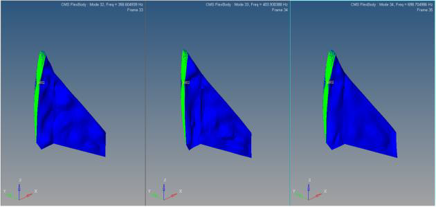
Review flexbody modes.
On successful completion of solver run, open the flexbody
flex_ForeCanard.h3d created from OptiStruct run in HyperView to review the various mode shapes. Your
flexbody contains 34 modes constituting normal modes, constraint modes,
and Static modes. Figure 32. Figure 33. Figure 34.
Create a MotionView Model
In this step, you will create a MotionView model of the
Fore Canard.
A MotionView model of the fore canard mechanism has
been provided. In this model, the Fore Canard body is modeled as a rigid body. In this
next step we will replace the rigid Fore Canard body with a flexible body created in the
previous step and use ModalForce entities to scale the pressure loads with respect to
canard position.
Open the ForeCanard_Model.mdl in MotionView. Review the model.
The model contains the following elements:
Four bodies namely Fore Canard, Torque Arm, Piston, and Cylinder.
A motion on the Piston with an expression 0.025*SIN(2*PI*TIME) to extend
and retract the piston by 25mm at 1 Hz. This piston motion varies the
fore canard angular position between -9.619 deg to +9.984 deg. Figure 35.
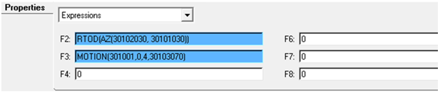
An expression type Output request to measure the “ForeCanard angular
position” and “Piston force along its axis”. The Fore canard angular
position is measured from the
RevJnt_TorqueArm_Gnd joint rotation
angle using the expression
`RTOD({j_4.AZ})`. The Piston force is
measured from the Piston Motion using the expression
`MOTION({mot_0.idstring},{0},{4},{j_2.i.idstring})`.
Figure 36.
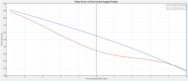
Solve the model with the rigid Canard to review piston forces without
aerodynamic loads.
Click the (Run) panel icon.
Specify the MotionSolve file name as
ForeCanard_withoutAeroloads.xml.
Specify the Simulation type as Quasi-static, the
End time as 1 second, and the Print interval as
0.01.
Click the Run.
After the simulation is complete, click the
Animate button to view the animation in
HyperView.
Figure 37.
On the Run panel in MotionView, click the
Plot button to load the
ForeCanard_withoutAeroloads.abf file in
HyperGraph 2D.
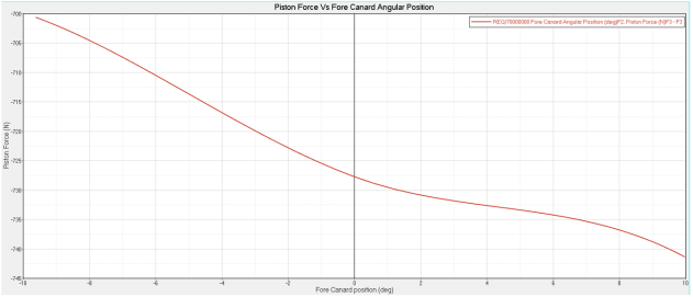
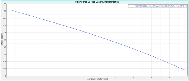
Use the data in Table 1and Table 2 to plot the Piston Force versus Fore Canard Angular
Position in HyperGraph.
Table 1.
X-axis Data
X Type
Expression
X Request
REQ/70000000 Fore Canard Angular Position
(deg)F2, Piston Force (N)F3
X Component
F2
Table 2.
Y-axis data
Y Type
Expression
Y Request
REQ/70000000 Fore Canard Angular Position
(deg)F2, Piston Force (N)F3
Y Component
F3
Figure 38.
Return to MotionView.
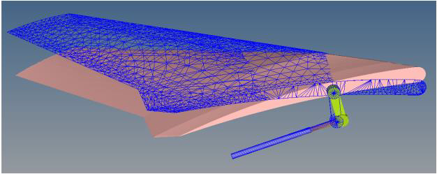
Switch the rigid fore canard to a flexible body.
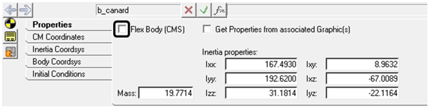
From the Project Browser, select the
Fore Canard body.
In the Body panel, activate the Flex Body(CMS)
check box.
Figure 39.
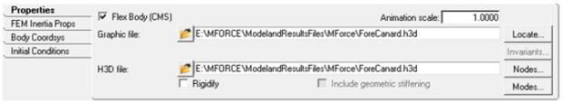
Browse your <working directory> and specify
flex_ForeCanard.h3d for the Graphic and H3D
files.
Figure 40.
Click the Nodes button and resolve the flexbody
interface nodes.
Model Aero-dynamic loads through Modal Force Entity.
The aero-dynamic loads are estimated at three distinct positions of canard
namely - 10 deg, 0deg, 10deg. Assume each pressure load to linearly vary in
interval ±10deg on a 0 to 1 scale. This variation of the aero-dynamic loads is
achieved by scaling Modal Forces with respect to canard angle using an
expression.
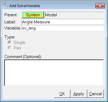
Right-click on the (SolverVariable) icon.
In the dialog, specify the Label as Angle
Measure and the Variable name as
sv_ang.
Figure 41.
Click OK.
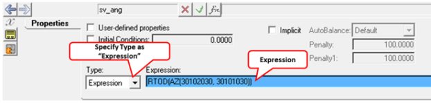
In the SolverVariable panel, under the Properties
tab, specify the Type as Expression and enter
`RTOD({j_4.AZ})` in the Expression
field.
Figure 42.
After completing steps 5.a through
5.d,
you have created an explicit variable that measures the fore Canard
angle.
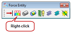
On the Force Entity toolbar, right-click on the (ModalForce) icon.
Figure 43.
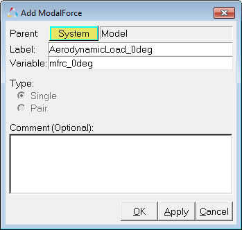
In the Add Modal Force dialog, specify the Label
as AerodynamicLoad_0deg and the Variable name as
mfrc_0deg.
Figure 44.
Click OK.
This will display the ModalForce panel.
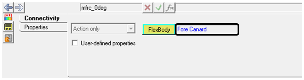
Configure the ModalForce panel.
In the Connectivity tab, specify Fore Canard for
the Flexbody.
Figure 45.
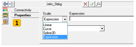
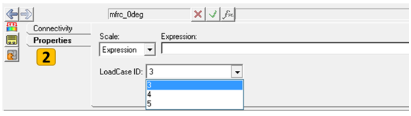
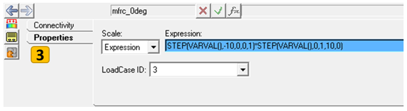
From the Properties tab, specify the Scale type as
Expression, the LoadCaseID as
3, and the Expression as
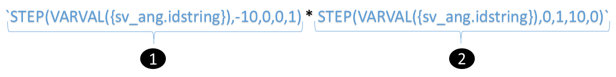
`STEP(VARVAL({sv_ang.idstring}),-10,0,0,1)*STEP(VARVAL({sv_ang.idstring}),0,1,10,0)`.
Figure 46. Figure 47. Figure 48.
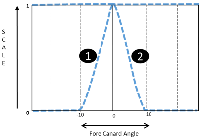
The product of the two STEP functions evaluates to gradually
increasing the value of the scale from 0 to 1 and then back to 0, while
the canard angular position varies from -10deg to 10 deg as shown in the
expression in Figure 49: Figure 49. Figure 50.
Follow steps .5.e through 6.b to
create the remaining Modal Forces as specified in Table 3:
 as the mode shapes of the flexible body, and
  as the Nodal load acting on the flexible body, the
equivalent Modal load on the flexible body
as the Nodal load acting on the flexible body, the
equivalent Modal load on the flexible body  is defined as:
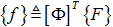
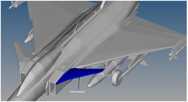
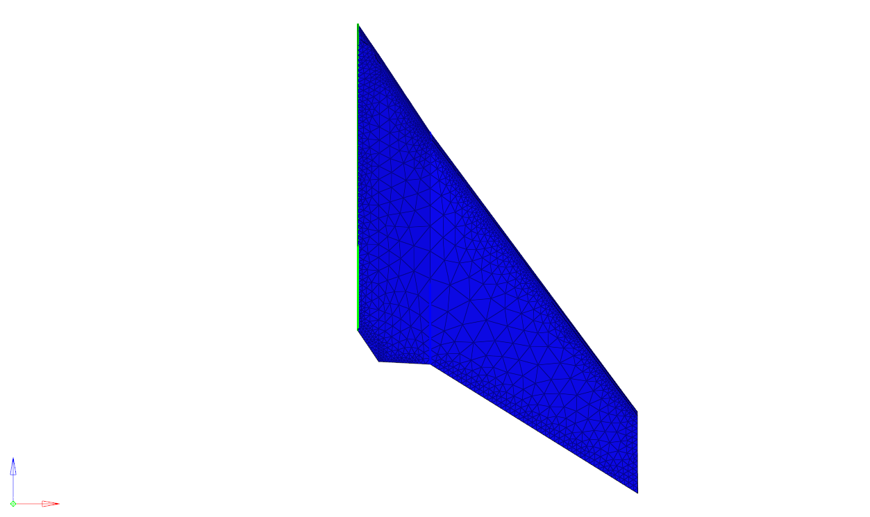
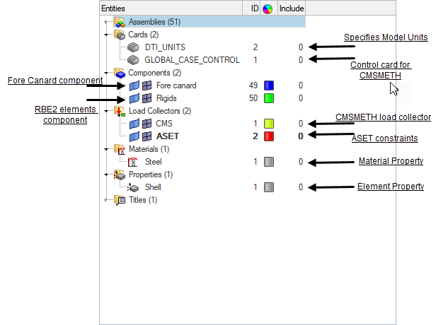
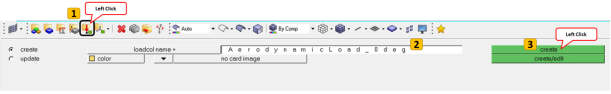

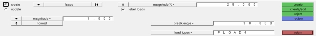

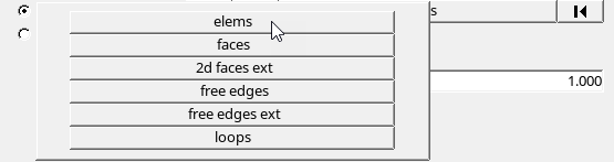

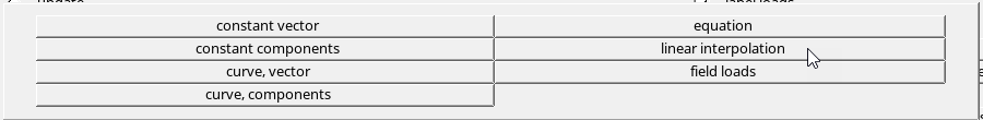
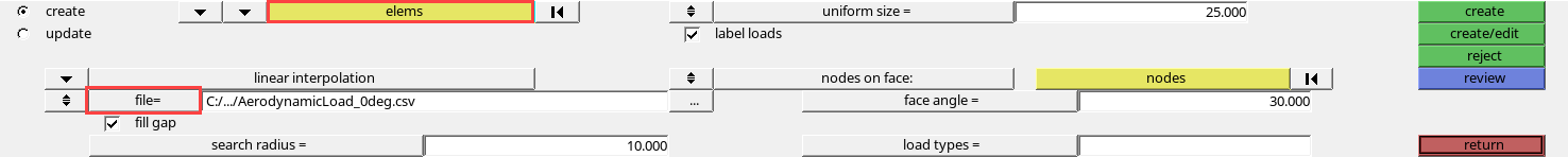 Figure 11.
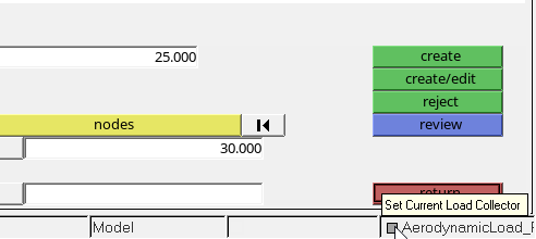


 (Run) panel icon.
 (SolverVariable) icon.
 (ModalForce) icon.
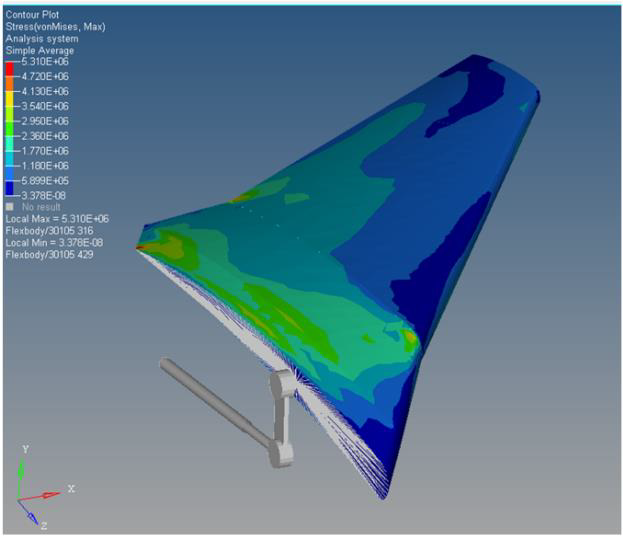
 (Start/Pause Animation) button
to play the animation.
(Start/Pause Animation) button
to play the animation. (Contour) panel button.