ACU-T: 5100 Modeling of a Fan Component: Axial Fan
Prerequisites
This simulation provides instructions for running a steady state simulation of flow inside a pipe with an interior fan placed at the middle of the pipe. Prior to starting this tutorial, you should have already run through the introductory HyperWorks tutorial, ACU-T: 1000 HyperWorks UI Introduction, and have a basic understanding of HyperWorks CFD and AcuSolve. To run this simulation, you will need access to a licensed version of HyperWorks CFD and AcuSolve.
Prior to running through this tutorial, copy HyperWorksCFD_tutorial_inputs.zip from <Altair_installation_directory>\hwcfdsolvers\acusolve\win64\model_files\tutorials\AcuSolve to a local directory. Extract ACU-T5100_AxialFan.hm and AxialCoefficient.csv from HyperWorksCFD_tutorial_inputs.zip.
Problem Description
The problem to be solved in this tutorial is shown schematically in the figure below. It consists of an interior fan which rotates at a speed of 377 rad/sec (~3600 RPM) and has a thickness of 0.06 m and a tip radius of 0.11 m. The volumetric flow rate at the inlet is 0.146 m3/sec (~525.35 m3/hr). The problem is simulated as a steady state run and the pressure rise across the fan region is computed.

Figure 1.
Start HyperWorks CFD and Open the HyperMesh Database
-
From the Home tools, Files tool group, click the Open Model tool.

Figure 2.The Open File dialog opens.
Validate the Geometry
The Validate tool scans through the entire model, performs checks on the surfaces and solids, and flags any defects in the geometry, such as free edges, closed shells, intersections, duplicates, and slivers.
Figure 3.
Set Up Flow
Set the General Simulation Parameters
-
From the Flow ribbon, click the Physics tool.

Figure 4.The Setup dialog opens. -
Under the Physics models setting:
- Verify that Time marching is set to Steady.
- Select Spalart-Allmaras as the Turbulence model.
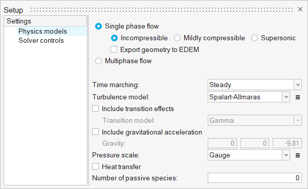
Figure 5. -
Click the Solver controls setting and verify that the
parameters are set as shown in the figure below.
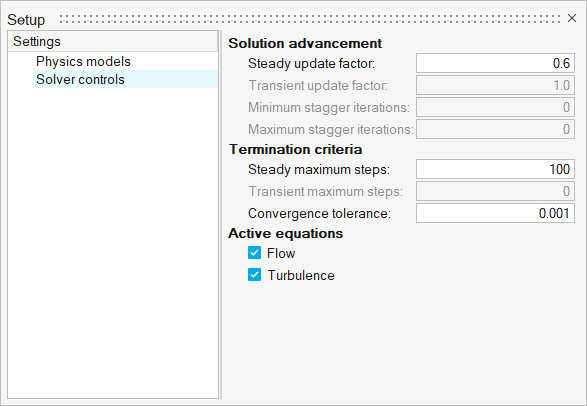
Figure 6.
Assign Material Properties
-
From the Flow ribbon, click the Material tool.

Figure 7. -
Click
 on the guide bar to exit the tool.
Define the Fan Component
-
From the Flow ribbon, click the arrow next to the
Domain tool set, then select
Fan Component.
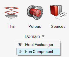
Figure 8. -
Select the middle solid as the fan component volume.
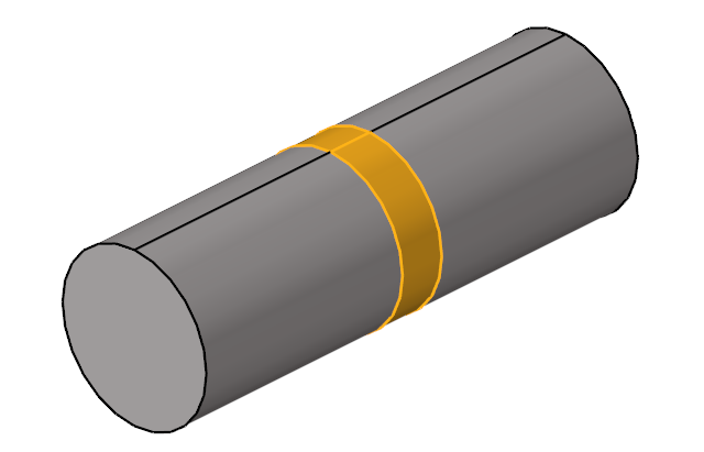
Figure 9. -
On the guide bar, click Surfaces
then select the face shown below as the inlet of the fan component.
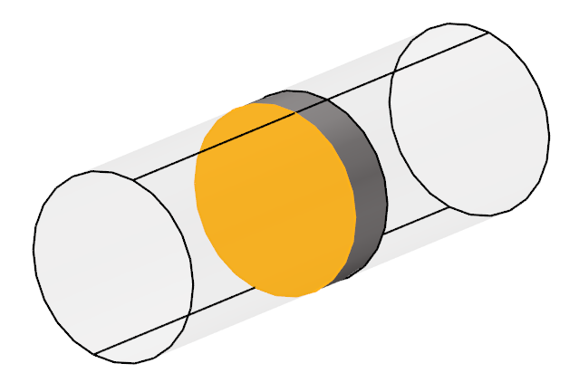
Figure 10. -
From the View Controls toolbar, change the geometry visualization mode from
Shaded Geometry to Transparent Geometry.
This allows you to view the axis direction vector in the next step.
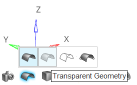
Figure 11. -
Click
 in the microdialog to flip the axis vector to the +X
direction.
in the microdialog to flip the axis vector to the +X
direction.
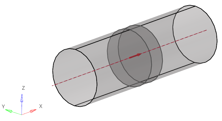
Figure 12. -
Enter 0.06 for Thickness.
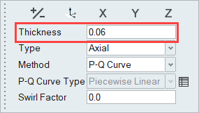
Figure 13. -
Click
 beside P-Q Curve Type to open
the Profile Editor.
beside P-Q Curve Type to open
the Profile Editor.
-
Click
 , browse to the location where
you saved AxialCoefficient.csv, and open it.
, browse to the location where
you saved AxialCoefficient.csv, and open it.
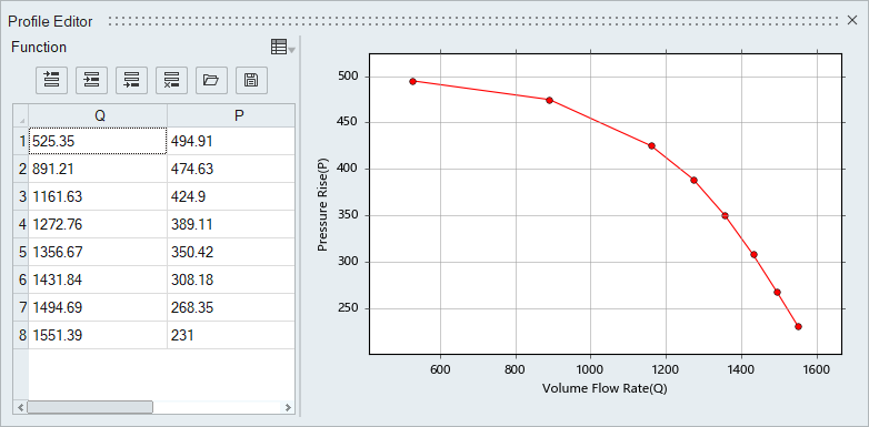
Figure 14. -
On the guide bar, click
 to execute
the command and exit the tool.
to execute
the command and exit the tool.
Define Flow Boundary Conditions
-
From the Flow ribbon, Profiled
tool group, click the Volumetric Flow Rate tool.

Figure 15. -
Click the inlet face highlighted in the figure below.
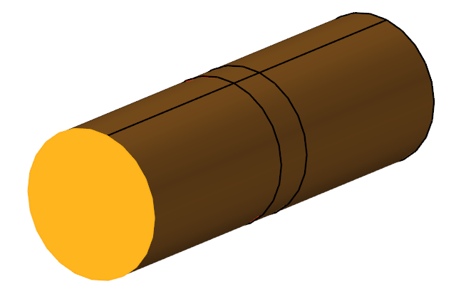
Figure 16. -
In the microdialog, enter 0.146
for the flow rate.
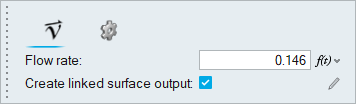
Figure 17. -
On the guide bar, click
to execute
the command and exit the tool.
-
Click the Outlet tool.

Figure 18. -
Select the face highlighted in the figure below and then click on the
guide bar.
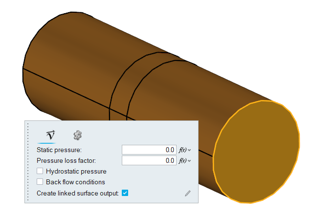
Figure 19.
Generate the Mesh
-
From the Mesh ribbon, click the Batch tool.

Figure 20. -
In the Meshing Operations dialog, set the Average element
size to 0.01 and the Mesh growth rate to
1.1 (if not set already).
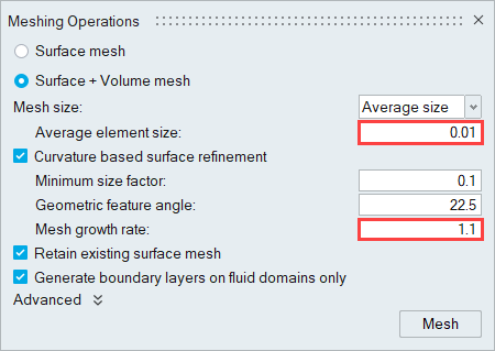
Figure 21.
Run AcuSolve
-
From the Solution ribbon, click the Run tool.

Figure 22.The Launch AcuSolve dialog opens. -
Leave the remaining options as default and click
Run to launch AcuSolve.
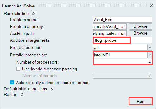
Figure 23.
Post-Process with AcuProbe
As the solution progresses, the AcuProbe window is launched automatically. AcuProbe can be used to monitor various variables over solution time.
-
Right-click on Final and select Plot
All.
Note: You might need to click
 on the toolbar in order to
properly display the plot.
on the toolbar in order to
properly display the plot.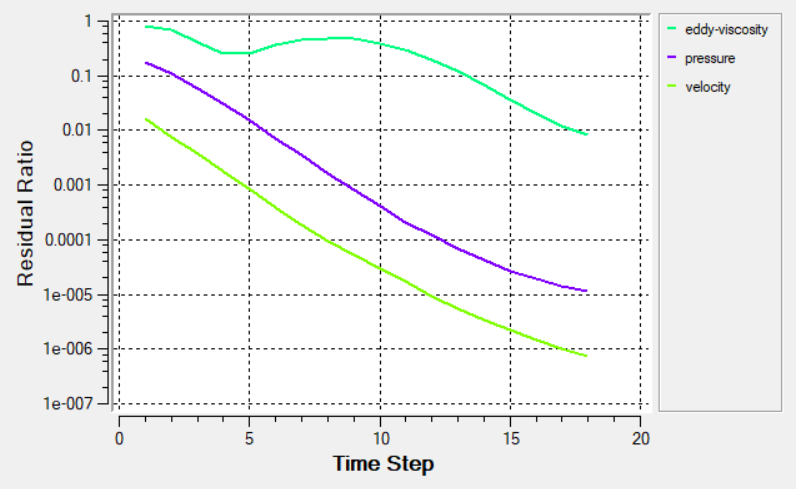
Figure 24. -
Click the User Function icon
 from the toolbar.
-
In the Function field of the User Function dialog, type
Fan_In = then paste the name you just copied.
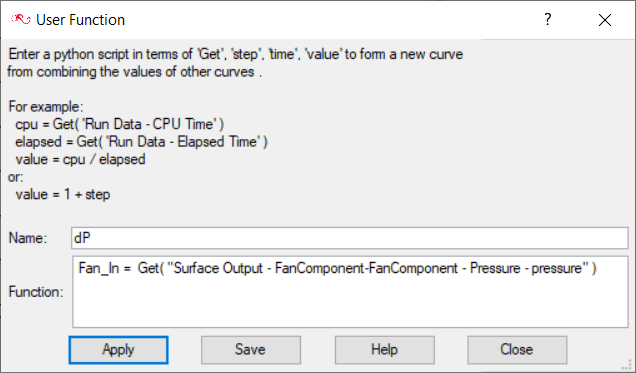
Figure 25. -
On a new line, type value = Fan_Out - Fan_In.
Note: The word “value” is case sensitive and should always be in lower case. If you use a capital letter, an error window appears.
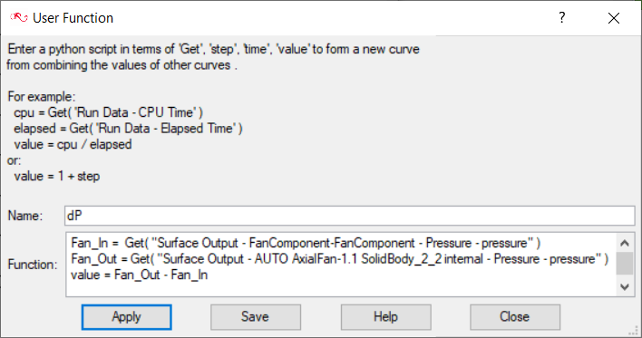
Figure 26. -
Click Apply.
As shown in the plot below, for the given problem, the pressure rise is 494.514 Pa.
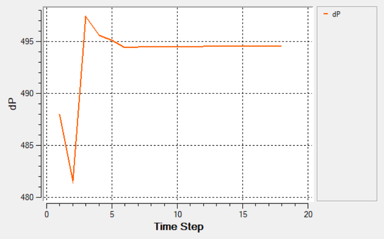
Figure 27.You can zoom into the plot by clicking
 then selecting an area at the end of the curve. As shown in the figure
below, for the given flow rate of 525.35 m3/hr (0.146
m3/sec), the pressure rise is 494.514 Pa.
then selecting an area at the end of the curve. As shown in the figure
below, for the given flow rate of 525.35 m3/hr (0.146
m3/sec), the pressure rise is 494.514 Pa.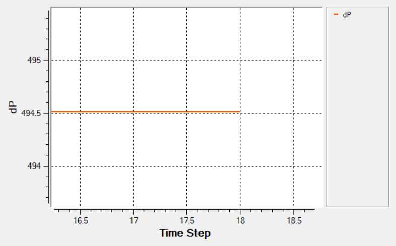
Figure 28.
Summary
In this tutorial, you successfully learned how to set up and solve a simulation involving a fan component using HyperWorks CFD. You imported the geometry and then defined the simulation parameters, fan component, and flow boundary conditions. Once the solution was computed, you defined a user-function in AcuProbe in order to create a plot of the pressure rise across the fan volume.